Quantisation Without Guesswork: What 4-Bit Models Save and What to Measure
SAMVIT Labs Research·6 min read
Model Research/Research review
A plain-language explanation of quantisation, group metadata and calibration, with reproducible storage arithmetic and a practical quality-testing plan.
On this page
ABOUT THE EVIDENCEThe quantiser and storage format in the figures are deliberately simplified analytical examples. They do not reproduce AWQ, GPTQ or a measured production model format.
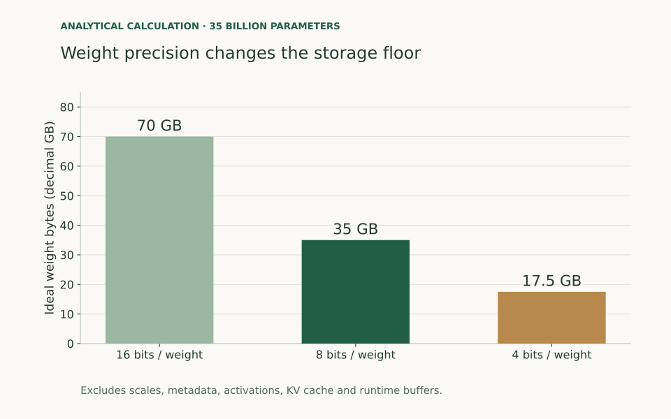
An eight-billion-parameter model needs sixteen decimal gigabytes if every weight occupies sixteen bits. Store each weight in four bits and the ideal payload falls to four gigabytes. That is an attractive starting point for running useful models on more modest hardware.
The word ideal matters. Real formats include scales, packing rules and sometimes higher-precision tensors. Running the model also needs memory for attention state, intermediate values and software buffers. Four-bit weights describe one part of the deployment, not the size of the whole process.
Quantisation is best treated as an engineering change with a quality budget. The aim is to reduce resource use while preserving the behaviour the application needs.
Replace many possible values with a smaller set
A trained weight is a number that helps determine the model’s output. Quantisation represents that number using a smaller set of possible values. A scale tells the runtime how to interpret the stored code.
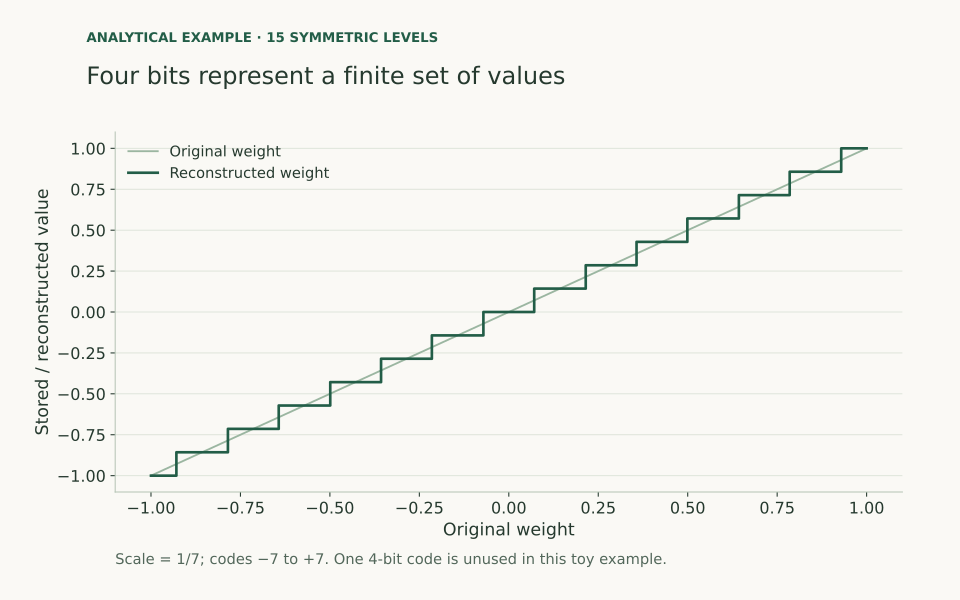
For a toy example, take weights between minus one and one. Set a scale s=1/7, round to an integer code and reconstruct the value:
q=clip(round(w/s),−7,7),w^=sq
This uses fifteen symmetric levels, leaving one of the sixteen possible four-bit codes unused. It is a teaching example, not the definition of a production four-bit format. A weight of 0.31 reconstructs to approximately 0.2857 because the stored code is two. The reconstruction error is about minus 0.0243.
Figure 1. A simplified symmetric quantiser. Nearby weights can share the same stored value. Real formats may use asymmetric ranges, learned scales or non-uniform codes. Download the example values.
Small numerical errors do not translate directly into the same percentage change in answer quality. Some operations tolerate approximation well; others amplify it. That is why file-size arithmetic needs to be followed by task evaluation.
Not every weight matters equally
The AWQ paper studies weight-only quantisation using activation information to identify important channels and choose scaling. Its central lesson is that simply rounding every weight with one global rule leaves useful information on the table. The deployment benefit depends on the matching inference implementation as well as the compressed values. [1]
GPTQ takes a different route: it uses approximate second-order information to reduce reconstruction error during post-training weight quantisation. Both are examples of methods that do more than save an array with fewer bits. Their published results belong to their tested models and hardware, not to every file carrying a four-bit label. [2]
A useful evaluation compares the same base checkpoint before and after compression. Changing the checkpoint, prompt template and quantisation method together makes it hard to identify which change caused a regression.
Account for the metadata
Many formats divide weights into groups. Each group shares metadata such as a scale or zero point. Smaller groups can represent local value ranges more closely, but they also need more metadata.
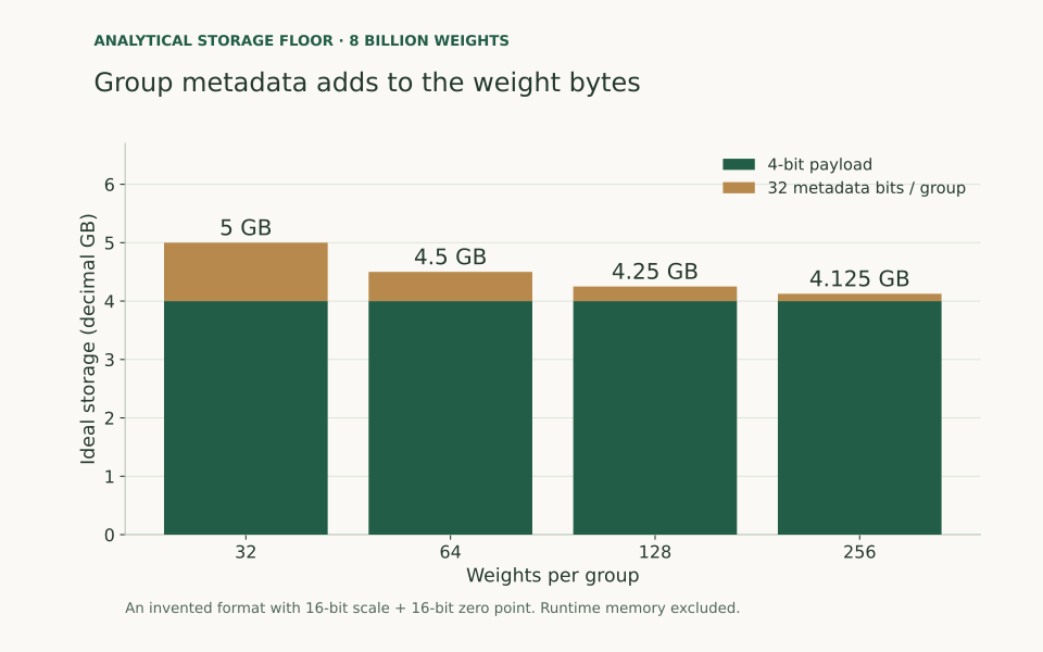
Consider an invented format containing four payload bits per weight and thirty-two metadata bits per group. If N weights divide exactly into groups of size g, the ideal byte count is:
M=8N×4+gN×832
For eight billion weights and a group size of 128, the payload is four decimal gigabytes and metadata adds 0.25 gigabytes. The total is 4.25 GB before headers, alignment, unquantised tensors and runtime memory. The effective storage is 4.25 bits per weight for this particular invented format.
Figure 2. Analytical metadata overhead for the stated format: one sixteen-bit scale and one sixteen-bit zero point per group. Actual formats make different choices. No runtime allocation is included. Download the calculation data.
Do not use the chart to choose a group size on quality grounds. It contains no quality measurements. Its purpose is to explain why the number on a model label can differ from the final file size.
Weight precision and activation precision are separate
A weight-only method can keep activations at higher precision. A different method may quantise both. SmoothQuant studies an eight-bit weight-and-activation approach by moving quantisation difficulty from activations toward weights through a mathematically equivalent transformation before quantisation. [3]
These distinctions affect kernel support and hardware efficiency. “INT4” is incomplete as a deployment description. Record what is four-bit, what remains in floating point and where dequantisation occurs.
The attention KV cache is another separate choice. Its memory grows with context length and concurrent sequences, so a compressed model can still run out of memory under a long-context workload. Measure peak resident memory for representative requests rather than adding up weight files alone.
Make calibration resemble the intended task
Some methods use calibration examples to choose compression parameters. Those examples should reflect the texts the model will process: document structure, language mix, typical context length and important domain terms.
A set of short general conversations may miss the activation patterns of long financial tables. Conversely, calibrating exclusively on one narrow template can give a misleading impression of broad quality. Keep calibration, tuning and final evaluation examples separate.
Maintain a small set of deliberately difficult cases: negative amounts, similar product identifiers, contradictory instructions and required abstentions. Add cases involving uncommon scripts or long inputs when the application needs them. Record the exact calibration dataset version so that a later build can be reproduced.
Evaluate useful outcomes before throughput
A practical comparison should answer several questions in order:
Check
Example measurement
What it can reveal
Output structure
Valid required fields and types
Formatting regressions
Task quality
Accepted extraction or classification result
Business-relevant changes
Important slices
Performance by language and document type
Concentrated failures
Abstention
Correct review routing on ambiguous inputs
Unsafe overconfidence
Serving behaviour
TTFT, completion latency and peak memory
Deployment cost and responsiveness
Stability
Repeated runs and load tests
Rare failures and queue pressure
Use paired examples so each configuration sees the same task. Review disagreements rather than relying only on an overall score. A model that loses one percentage point on a broad benchmark may lose much more on the particular field your application uses.
Finally, measure the actual runtime on the target device. Lower weight precision can reduce memory traffic, but packing, conversion and unsupported kernels can consume some of the gain. Report the serving engine, hardware, batch size, context lengths and model format with the result.
The useful deliverable is a tested configuration: a particular checkpoint, compression recipe, runtime and acceptance record. A small file becomes a practical product component only when that complete configuration works for its intended task.
The SAMVIT Labs research and engineering journal. We examine model efficiency, practical agent workflows and the evidence needed to make informed deployment decisions.